Call:
glm(formula = Draw_dummy ~ Avg_Goals_For_Home + Avg_Goals_Against_Away +
    Avg_Goals_Against_Home + Avg_Goals_For_Away, family = binomial(link = "logit"),
    data = df)

Coefficients:
                       Estimate Std. Error z value Pr(>|z|)
(Intercept)            -0.86441    0.16896  -5.116 3.12e-07 ***
Avg_Goals_For_Home      0.10666    0.04567   2.335 0.019527 *
Avg_Goals_Against_Away  0.17576    0.05269   3.335 0.000852 ***
Avg_Goals_Against_Home -0.07225    0.05294  -1.365 0.172299
Avg_Goals_For_Away     -0.04832    0.04723  -1.023 0.306227
---
Signif. codes:  0 '***' 0.001 '**' 0.01 '*' 0.05 '.' 0.1 ' ' 1

(Dispersion parameter for binomial family taken to be 1)

    Null deviance: 9532.3  on 7340  degrees of freedom
Residual deviance: 9489.2  on 7336  degrees of freedom
AIC: 9499.2

Number of Fisher Scoring iterations: 4Home, away and interaction effects of Goals
Analysis
Is there a an interaction effect between goals for and against when predicting for draws?
TLDR
- There are 3 significant effects in predicting draws:
- Average Goals Against x Away
- Average Goals For x Home
- Interaction between ‘Average Goals Against x Away’ & ‘Average Goals For x Home’
- Alone, they have very limited predictive power for draws
Model so far
So far the best model to predict for draws in the Eredivisie includes a team’s for and against goals. Goals for and against speak to a team’s ability to stop opponents from scoring as well as their own ability to create goals. Below I’ll explore this a bit more by testing for
home and away effects on draws
interactive effect on draws
I’m going to break up the goals for and against by bringing in a home and against dimension. The idea is that playing home or away has an effect and therefore it has an effect on a team’s ability to create and concede goals.
| For goals | Against goals | |
| Home goals | For x Home goals | Against x Home goals |
| Away goals | For x Away goals | Against x Away goals |
To make things even more complicated, there’s also interaction effects I will test for. A normal regression takes variables and estimates the effects of those variables – for example, the effect of goals for and against on the chances of a draw. Sometimes the interaction of the prediction variables (for and away goals) have effects on each other. These are called interaction effects.
We can pipe both into a regression to see if and how much they affect the home team’s chances of winning. However, if we’d do only that we’d be missing a third effect: the effect that home and scoring-ability have on each other. This third effect is the interaction effect. It would measure how much a high or a low scoring-ability effects the home-team effect.
Let’s build a model from the ground up and compare them against each other
The base model above uses all 4 goal types from the quadrant as predictors for the odds of a game turning into a draw. So we’re calculating how and if the goal types predict for draws, as independent effects. This means we’re not yet interesting in these effects interacting with each other.
Note that I’ve used a team’s average goals up until a match is played to predict for draws.
The output teaches us:
3 significant effects:
The intercept
- The odds are initially low for a draw at -0.86441
Average Goals Against x Away
For every +1 average goal, add 0.10666 to the intercept
A team’s average of goals conceded during away-games increases the chances of a draw
Average Goals For x Home
For every +1 average goal, add 0.17576 to the intercept
A team’s average of goals created during home-games increases the chances of a draw
This is quite the revelation because of what isn’t significant
The home team’s average goals against and the away team’s average goals for are not good predictors for draws! Let’s work this into a model that includes an interaction effect.
Call:
glm(formula = Draw_dummy ~ Avg_Goals_For_Home * Avg_Goals_Against_Away +
    Avg_Goals_Against_Home + Avg_Goals_For_Away, family = binomial(link = "logit"),
    data = df)

Coefficients:
                                          Estimate Std. Error z value Pr(>|z|)
(Intercept)                               -1.75304    0.24580  -7.132 9.89e-13
Avg_Goals_For_Home                         0.61353    0.11194   5.481 4.23e-08
Avg_Goals_Against_Away                     0.67993    0.11462   5.932 2.99e-09
Avg_Goals_Against_Home                    -0.05696    0.05325  -1.070    0.285
Avg_Goals_For_Away                        -0.03111    0.04758  -0.654    0.513
Avg_Goals_For_Home:Avg_Goals_Against_Away -0.29602    0.06041  -4.901 9.56e-07

(Intercept)                               ***
Avg_Goals_For_Home                        ***
Avg_Goals_Against_Away                    ***
Avg_Goals_Against_Home
Avg_Goals_For_Away
Avg_Goals_For_Home:Avg_Goals_Against_Away ***
---
Signif. codes:  0 '***' 0.001 '**' 0.01 '*' 0.05 '.' 0.1 ' ' 1

(Dispersion parameter for binomial family taken to be 1)

    Null deviance: 9532.3  on 7340  degrees of freedom
Residual deviance: 9462.8  on 7335  degrees of freedom
AIC: 9474.8

Number of Fisher Scoring iterations: 4
Analysis of Deviance Table
Model 1: Draw_dummy ~ Avg_Goals_For_Home + Avg_Goals_Against_Away + Avg_Goals_Against_Home +
Avg_Goals_For_Away
Model 2: Draw_dummy ~ Avg_Goals_For_Home * Avg_Goals_Against_Away + Avg_Goals_Against_Home +
Avg_Goals_For_Away
Resid. Df Resid. Dev Df Deviance Pr(>Chi)
1 7336 9489.2
2 7335 9462.8 1 26.341 2.862e-07 ***
---
Signif. codes: 0 '***' 0.001 '**' 0.01 '*' 0.05 '.' 0.1 ' ' 1For this model I only added an interaction effect between Average Goals Against x Away and Average Goals For x Home. And would you look at that: we’ve got an improved model and a significant interaction effect. A quick summary of the output before I visualize it:
4 significant effects:
The intercept
- The odds are initially even lower for a draw at -1.75304
Average Goals Against x Away
For every +1 average goal, add 0.61353 to the intercept
A team’s average of goals conceded during away-games increases the chances of a draw
Average Goals For x Home
For every +1 average goal, add 0.67993 to the intercept
A team’s average of goals created during home-games increases the chances of a draw
Interaction between ‘Average Goals Against x Away’ & ‘Average Goals For x Home’
- When both goal-types go up, the odds of a draw decreases by -0.29602
Importantly, the interaction variable changes the model outcomes a lot
In the new model, a draw is even less likely (the intercept) and the interaction effect becomes the only significant effect that makes it even ‘less-less’ likely to draw. This means that in absence of an interaction effect, the two goal-types become positive until they interact with each other and teams are so “goal-happy” together that matches are less likely to draw.
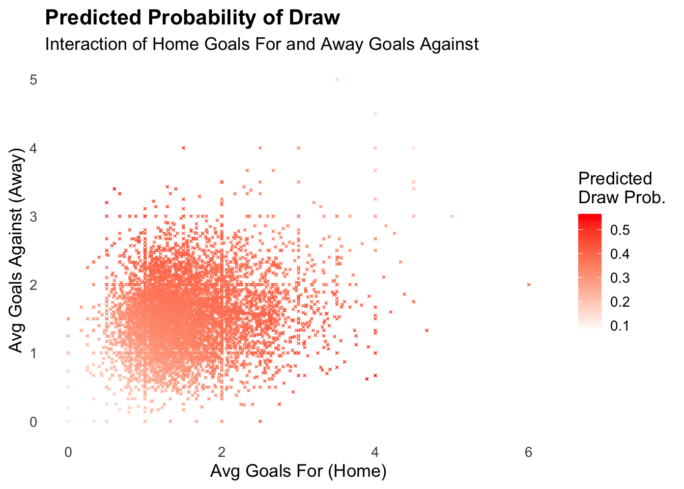
A visual to illustrate. Note that the chart shows predictions to be in a sweet spot of an average of between 1-2 for both goal types, and that more of both (the empty space >3) gets us into interaction area of too much of both goal types.
As we have an improved model now, let’s as a last exercise compare predictions using this model to actual outcomes. After all, I’m sitting on years of Eredivisie data so I can use the model to predict odds for a draw for each match, and then see how close I am to predicting correctly.
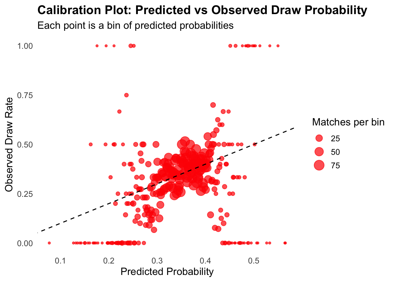
The visual paints a picture of predicted vs actual draws with broad brushes. Importantly the diagonal line represents the line of perfect calibration where predicted = observed. So ideally all dots line up on that line. Visually I notice:
there’s plenty of action on or near the line, but also away from the line
so for sure this model is not a perfect or even a good predictor
But let’s be more precise
Let’s get some hard numbers on how accurate the model predicts by creating a confusion matrix. This will show how many true and false positives the model predicts for. We want the model to be better than flipping a coin so I’m setting this as a standard: the model needs to predict correctly in more than 50% of the time.
Confusion Matrix and Statistics

          Reference
Prediction    0    1
         0 4743 2585
         1    7    6

               Accuracy : 0.6469
                 95% CI : (0.6359, 0.6579)
    No Information Rate : 0.6471
    P-Value [Acc > NIR] : 0.5151

                  Kappa : 0.0011

 Mcnemar's Test P-Value : <2e-16

            Sensitivity : 0.0023157
            Specificity : 0.9985263
         Pos Pred Value : 0.4615385
         Neg Pred Value : 0.6472434
             Prevalence : 0.3529492
         Detection Rate : 0.0008173
   Detection Prevalence : 0.0017709
      Balanced Accuracy : 0.5004210

       'Positive' Class : 1
The most important parts of the output above are:
the matrix between predicted and reference (actual)
it’s virtually always right for 0 - 0
i.e. for getting true negatives right
high specificity
it’s virtually always wrong for getting 1 - 1
i.e. for getting true positives right
low sensitivity
For good measure a visual showing how much better this model is than using a coin-flip
Setting levels: control = 0, case = 1Setting direction: controls < cases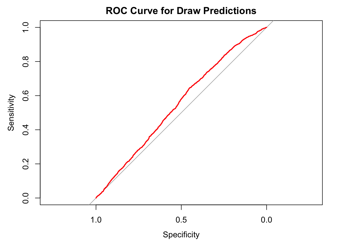
In conclusion
I’ve identified some significant effects but this model needs improving to have any predictive power. There are many other variables still to test for which could improve this model so we have something here that can and should only get better as I identify more variables with predictive power.